Difference between revisions of "TimeSeriesMapping/hydrology/en"
BhawaniRegmi (Talk | contribs) (→Time Series Area Models ("GM")) |
BhawaniRegmi (Talk | contribs) (→Time Series Area Models ("GM")) |
||
| Line 30: | Line 30: | ||
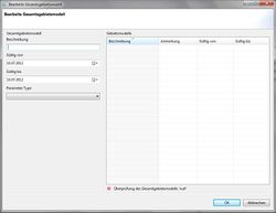
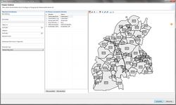
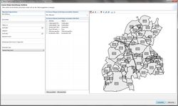
[[File:Zeitreihenzuordnung Bearbeite Gebietsmodell.jpg|thumb|250px|Dialog to create new ("New Area Model (Linear sum)") or editing a Time Series Area Model type ''Linear Sum'']] | [[File:Zeitreihenzuordnung Bearbeite Gebietsmodell.jpg|thumb|250px|Dialog to create new ("New Area Model (Linear sum)") or editing a Time Series Area Model type ''Linear Sum'']] | ||
; Linear Sum | ; Linear Sum | ||
| − | : Combine a multiple output time series [[Zeitreihen/hydrology/de|Time Series Management]] over linear factors for Time Series Area Model. For each time step ''i'' a Time Series Area Model is calculated as follows: ''tg (i) = sum (fn * tzn (i))'' with: | + | : Combine a multiple output time series [[Zeitreihen/hydrology/de|Time Series Management]] over linear factors for Time Series Area Model. For each time step (''i'') a Time Series Area Model is calculated as follows: ''tg (i) = sum (fn * tzn (i))'' with: |
:* ''tg'' the area time series, | :* ''tg'' the area time series, | ||
:* ''i'' the time step, | :* ''i'' the time step, | ||
Latest revision as of 22:09, 17 February 2017
Contents |
[edit] Mapping of Time Series
The Model Management of KalypsoHydrology is enhanced by the configuration and management to generate area-based time series (in German: “Gebietsmodell” = GM). A GM in a general sense is the generation of a time series of a sub-catchment (for example, precipitation). In addition, there is still the possibility for certain types of data (for example, flow) is a direct correlation between time series and defined model elements (for example, node).
The time series assignments are defined independently of the simulation and can be used in different combination. The time series assignment is used as input data, from the Time series management. A defined assignment can be reused for the generation of any calculation variants. The previously (till Kalypso version 12) required time-consuming manual assignment of sub-catchments to (Precipitation, Temperature and Evaporation) time series are deleted. When you create a simulation variation the user assigns time series arrangements. For each simulation, a set of time-series arrangements GM(such as Precipitation, Evaporation, Temperature, Flows etc.) must be indicated. The data time series (for example, Rainfall) are generated during the computing time and automatically stored within the simulation data and the references.
Since the assignments are re-evaluated for each simulation, changes to the underlying time series within the time series management (for example, extending a time series, correction of individual values, etc.) are automatically updated.
In the Time series Managements view, the creation of new models or time series arrangement are carried out. For the possible arrangements, the type of arrangement from the list for the time series can be selected:
- Area models - Grass evaporation [mm]
- Area models - Medium temperature [° C]
- Area models - Precipitation [mm]
- Time series assignment – water level measurement
- Time series assignment - open water evaporation
- Time series assignment - inflow node
[edit] Simple Time Series Assignment
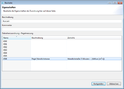
In a simple time series arrangement (Water level hydrographs, inflows and open water evaporation) is carried out at a one-to-one mapping between a time series from the Time Series Assignment and a model element. During the new time series assignment or when editing a time series assignment at any model element (for example, water level measurement is assigned to a model node ) is shown by a dialogue, in which all elements are listed in a table. By double-clicking in the second column of the table, the attributable time series can be selected.
[edit] Time Series Area Models ("GM")
A Time Series Area Model defines the mapping of (Precipitation) time series with a sub catchment. It can be generated in different ways.The following methods are implemented currently in Kalypso:
- Linear Sum
- Combine a multiple output time series Time Series Management over linear factors for Time Series Area Model. For each time step (i) a Time Series Area Model is calculated as follows: tg (i) = sum (fn * tzn (i)) with:
- tg the area time series,
- i the time step,
- tz1 bis tzn the input (measurement) time series and
- f1 bis fn whose linear factors
- Total Time Series Area Model
- (Temporal) combination of several (sub) –catchment models. For the formation of long-term Time Series Area Models for the long-term calibration a simple domain model is not sufficient, because the incoming (measurement) data may not be fully available for longer periods (reading failures, construction and conversion of stations, etc.). For this purpose, a validity period are assigned to each Time Series Area Model (optional). A variable surplus time for the total area of the model can then be defined by combining a plurality of such Time Series Area Model.
- Thus, the defined total area of the model can be used like a normal Time Series Area Model to generate a computational variant. For a total Time Series Area Model found in the formation of an area time series for each time step the current Time Series Area Model (GM)can be used.
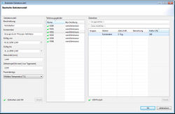
The Actions New Time Series Area Model (Linear sum) or New Total Time Series Area Model are respectively applied to new Time Series Area Models in which the user can edit all parameters in detail. When editing a Time Series Area Model via the appropriate action in the view of properties of the Time Series Area Model, the same editing options appear.
| The input fields of Time step [min] and Timestamp [hh: mm: ss] (only daily data) must be completed in the dialogue by Edit the Time Series Area Model (see Figure view New Time Series Area Model (Linear sum)), otherwise later the simulation cannot be completed. At a time stamp of 7:30 (e.g. for DWD data), the values are one daily dates. For another time stamp, the data is used for the specified day. |
| Time Series Area Models of grass evaporation and mean temperature are created only once for the long-term and short-term simulation variations with the daily value timestamp. |
[edit] Automatic determination of the linear factors for Time Series Area Models
In addition to the manual entry of the linear factors and arrangement carried out at the stations of the measurement, currently two methods are available:
- Determine the linear factors with the Thiessen method
- With the Thiessen method, the Thiessen polygons are determined for each station. The linear factors for a sub-catchment are then calculated from the area-weighted proportion of the overlapping of each Thiessen polygon with the proportional sub-catchment area.
- Determine the linear factors with the IDW method
- The inverse distance method (Inverse Distance Method) determines the linear factors first by n next stations assigned to a sub-catchment. The linear factors are then calculated in each case according to the partition of the distance between sub-catchment and the stations.
- The modeller can select how many stations (= 'n') to be used as maximum for the IDW method per sub-catchments.
The user can select which time series are to be taken into account for determining the linear factors in both processes. In both methods, the sum of the linear factors for each sub-catchment is normalized to 1 (= 100%).
| The fields valid from and valid to in the dialogue of the Thiessen method (see Figure view to View to "New Time Series Area Model (Linear sum) by Thiessen method" are required. It should be checked whether, the stored time series data covered by all stations are valid for the calculation time (validity). The alternative is an overall Time Series Area Model of multiple area models to be created in order to optimally utilize the available time series. |
| Language: | English |
|---|
